23 Sep Is pvalue.io reliable?
First of all, it is important to be aware that no statistical software guarantees the results it provides, even the most widely used software (including Excel).
pvalue.io is still new. It is a graphical interface to R, which is a reference statistical analysis software, as well as SAS, Stata and SPSS.
To produce and display the results, pvalue.io uses two extensions of R (packages) which are open source, therefore totally transparent, allowing everyone to check the quality of the code.
These two extensions are as follows:
– shiny, which allows to create graphical user interfaces
– simplestats, which contains high-level functions to simplify the presentation of results. This package determines the tests to be performed, the appropriate statistical models, the covaraites, and which displays figures and tables. In other words, simplestats controls the logic of pvalue.io.
Here we propose you to carry out a comparison of the results of analysis on R and on pvalue.io. To reproduce the results it is necessary to use the file described on the next page.
Univariable Analysis
Is the age different by gender? Welch T test
Results obtained with R
1 2 3 4 5 6 7 8 9 10 11 12 13 | tab <- readxl::read_excel("colon.xlsx") t.test(age ~ sex, data = tab) #> #> Welch Two Sample t-test #> #> data: age by sex #> t = -0.65672, df = 909.85, p-value = 0.5115 #> alternative hypothesis: true difference in means is not equal to 0 #> 95 percent confidence interval: #> -2.060734 1.027388 #> sample estimates: #> mean in group 0 mean in group 1 #> 59.48539 60.00207 |
Result reported by pvalue.io

Occlusion as a function of adherence: Chi2 test
Results obtained with R
1 2 3 4 5 6 | tab <- readxl::read_excel("colon.xlsx") chisq.test(table(tab$obstruct, tab$adhere), correct = FALSE) #> #> Pearson's Chi-squared test #> #> data: table(tab$obstruct, tab$adhere) #> X-squared = 0.18841, df = 1, p-value = 0.6642 |
Result reported by pvalue.io

Multivariable analysis
Logistic regression
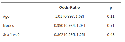
Influence of age, sex, adenopathy on organ adherence
Results obtained with R
1 2 3 4 5 6 7 8 9 10 11 12 13 14 15 16 17 18 19 20 21 22 23 24 25 26 27 28 29 30 31 32 33 34 35 36 37 | tab <- readxl::read_excel("colon.xlsx") mod <- glm(adhere ~ age + sex + nodes, family = binomial, data = tab) summary(mod) #> #> Call: #> glm(formula = adhere ~ age + sex + nodes, family = binomial, #> data = tab) #> #> Deviance Residuals: #> Min 1Q Median 3Q Max #> -0.6792 -0.5829 -0.5494 -0.5022 2.2344 #> #> Coefficients: #> Estimate Std. Error z value Pr(>|z|) #> (Intercept) -2.456604 0.536892 -4.576 4.75e-06 *** #> age 0.013148 0.008255 1.593 0.111 #> sex -0.148687 0.188682 -0.788 0.431 #> nodes -0.010391 0.027595 -0.377 0.707 #> --- #> Signif. codes: 0 '***' 0.001 '**' 0.01 '*' 0.05 '.' 0.1 ' ' 1 #> #> (Dispersion parameter for binomial family taken to be 1) #> #> Null deviance: 753.86 on 910 degrees of freedom #> Residual deviance: 750.42 on 907 degrees of freedom #> (18 observations deleted due to missingness) #> AIC: 758.42 #> #> Number of Fisher Scoring iterations: 4 exp(coef(mod)) #> (Intercept) age sex nodes #> 0.08572554 1.01323530 0.86183868 0.98966293 exp(confint(mod)) #> Waiting for profiling to be done... #> 2.5 % 97.5 % #> (Intercept) 0.02912675 0.2397119 #> age 0.99721763 1.0300594 #> sex 0.59483684 1.2479149 #> nodes 0.93435402 1.0415777 |
Result reported by pvalue.io

Survival analysis : Cox Model
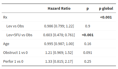
Influence of treatment, age, presence of bowel obstruction and occlusion on progression-free survival
Results obtained with R
1 2 3 4 5 6 7 8 9 10 11 12 13 14 15 16 17 18 19 20 21 22 23 24 25 26 27 28 29 30 31 32 33 34 35 36 37 38 39 40 41 42 43 | library(survival) tab <- readxl::read_excel("colon.xlsx") tab$rx <- as.factor(tab$rx) tab$rx <- relevel(tab$rx, ref = "Obs") mod <- coxph(Surv(time, progression_death) ~ rx + age + obstruct + perfor, data = tab) summary(mod) #> Call: #> coxph(formula = Surv(time, progression_death) ~ rx + age + obstruct + perfor, #> data = tab) #> #> n= 929, number of events= 468 #> #> coef exp(coef) se(coef) z Pr(>|z|) #> rxLev -0.013997 0.986101 0.107082 -0.131 0.8960 #> rxLev+5FU -0.505755 0.603050 0.118677 -4.262 2.03e-05 *** #> age -0.005514 0.994501 0.003918 -1.408 0.1593 #> obstruct 0.194194 1.214332 0.114925 1.690 0.0911 . #> perfor 0.285605 1.330566 0.250238 1.141 0.2537 #> --- #> Signif. codes: 0 '***' 0.001 '**' 0.01 '*' 0.05 '.' 0.1 ' ' 1 #> #> exp(coef) exp(-coef) lower .95 upper .95 #> rxLev 0.9861 1.0141 0.7994 1.216 #> rxLev+5FU 0.6031 1.6582 0.4779 0.761 #> age 0.9945 1.0055 0.9869 1.002 #> obstruct 1.2143 0.8235 0.9694 1.521 #> perfor 1.3306 0.7516 0.8148 2.173 #> #> Concordance= 0.572 (se = 0.013 ) #> Likelihood ratio test= 31.43 on 5 df, p=8e-06 #> Wald test = 30.12 on 5 df, p=1e-05 #> Score (logrank) test = 30.64 on 5 df, p=1e-05 anova(mod) #> Analysis of Deviance Table #> Cox model: response is Surv(time, progression_death) #> Terms added sequentially (first to last) #> #> loglik Chisq Df Pr(>|Chi|) #> NULL -3040.3 #> rx -3028.1 24.3435 2 5.175e-06 *** #> age -3026.8 2.5853 1 0.10786 #> obstruct -3025.2 3.3071 1 0.06898 . #> perfor -3024.6 1.1991 1 0.27349 #> --- #> Signif. codes: 0 '***' 0.001 '**' 0.01 '*' 0.05 '.' 0.1 ' ' 1 |
Result reported by pvalue.io


No Comments